Excel: Convert 4/28/2012 10:01:28 AM to 04-2012 Format Using Formulas & Next Cell Techniques

Hello,

My date format is: 4/28/2012 10:01:28 AM.
How to remove the day and time from the cell so that the date 04-2012 is created?
It's not that it doesn't appear, it just disappears.
Ev. what formula to use to make 04-2012 appear in the next cell.
= DATE (YEAR .... does not help.
Have any ideas?

PS. sorry but i'm not an advanced user of excel, google doesn't help me either.

Right click on the cell-> cell format-> custom and type with your finger or find in the list -> this: "mmm-ry"

It's not about not showing up, just that everything just disappears.
When I use the formatting, the value remains and only will not be displayed.
Then I have to make a graph of it, so I only need a month and a year

If the date will be in A1 and only 04-2012 is to be displayed then:
= MONTH (A1) & "-" & YEAR (A1)

But this will not necessarily work for a given chart (It depends what chart and what it really is supposed to represent).

Let me give you a hint that you'd better use custom formatting (as advised by my colleague pitermxa [only mm-yyyy or m-yyyy] ) and do the same formatting for this data in the graph (right-click on a given axis with dates in the chart and number format and set custom to mm-yyyy or m-yyyy there)

Enclosed is an example in two versions with a simple diagram.

Thanks a lot, formula = MONTH (A1) & "-" & YEAR (A1) works
but I have another problem because I can't format these cells and the date is 5-2012 and I would like it to be 05-2012 because later in the pivot table I get a mess. Can you do something about it?

Added after 2 [minutes]:

file in attachment

BTW. to moderators, maybe it's time to allow adding * .xlsx files?

do something like this
= (IF (MONTH (A2)

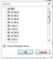
ok thanks but in the pivot chart I still have 5-2012, 3-2011 etc. moreover, how to sort by dates from the newest in the chart?

copy this column and paste only the values from this column and on its basis then make a pivot table and it should be ok

the blood sausage comes out, see 2010, on 9-2010, when it copies the content, excel does not convert it to a date (probably because the day is missing)

maybe to add to each month the day 01-05-2012, for example, so that excel would treat it as a date?

yes, but then it will sort by day of each year and the point is that it should sort chronologically, by date


and the date must necessarily be in this format?
I did something like this

thanks for the effort but the date is still not sorted.
I have to do this report once a week, and it better looks professional.
Thank you for all your help, I will keep looking.

The trouble is you want to "have a cookie and eat a cookie"
First you get rid of the date and then you want to make it again (adding 1). It does it differently, only it won't be useful to you.

For Excel, subsequent dates are consecutive numbers, starting from 1 for 01/01/1900, 2 for 02/01/1900 etc. The fact that you see it as a date is what you owe to the formatting.
Unfortunately, the data cannot be formatted in the pivot itself, so you can see what the standard format for the date is set to (if the data is a date, you see year-month-day, otherwise you see a text string or numbers).

If you want to group data after a month, you have to make concessions.
The formula below (and the above) changes the date to a string similar to a date, but it is not a date (and "adding" a one to it will not change that either - it will still be a text string, not a date).
The sorting of such data is therefore carried out according to the principle of text strings. In this case, the solution is to change the formula so that it shows first the year and then the month, ie: 2011-09

Then you will have the order (the order of "dates" consistent with the order in the text string).

= IF (MONTH (A2)

Cool, the last tip works great. Thanks a lot for contributing