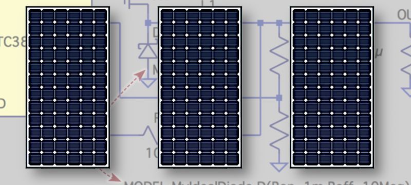
Like all other electronic components, it is possible to model a solar panel in a SPICE (Simulation Program with Integrated Circuit Emphasis) model. There are several ways to model a solar panel in SPICE, but one of the most common is to use a “current-voltage (I-V)” model to represent the relationship between the current produced by the solar panel and the voltage at its terminals. To create an I-V model, it is necessary to know the current and voltage values of the solar panel under different conditions, such as incident light intensity and panel temperature. In this article, we analyze these aspects.
Electrically modelling a solar panel
The electronic market makes thousands of solar panel models available to users. Each solar panel has its own electrical, physical and optical characteristics, so it is not possible to unify all the behaviors of such generators in one ideal device. One of the best methods to outline the electrical behavior of one’s solar panel is to collect measured experimental data to create a mathematical model. A solar panel does not have linear behavior, so the difficulty in generating the relevant equations may be greater. On the contrary, the solar panel is a highly non-linear element, so its behavior is comparable to a hybrid current generator (when the panel generates a low voltage due to strong loads) and a current generator (when the panel generates higher voltages due to light loads). It is therefore completely incorrect to equate the operation of a solar panel with a simple battery. For our analysis, we use a solar panel characterized by the following technical data:
• Maximum power: 250 W
• Open-circuit voltage: 37.8 V
• Short-circuit current: 8.7 A
• Maximum power voltage: 31.5 V
• Maximum power current: 7.94 A
• Module efficiency: 15.3%
• Operating temperature: between –40˚C and 85˚C
• Dimensions: 1,650 × 992 × 40 mm
• Weight: 17 kg
Figure 1 shows the graph of the current on the characteristic voltage. These values can also be deduced from practical measurements, with certain resistive loads applied to the solar panel itself. As shown in the figure, there are three separate graphs for three conditions under which the device is illuminated by the sun:
• 1,000 W/m2
• 800 W/m2
• 200 W/m2
The three curves can be summarized in as many mathematical models, which accurately express the course of current values as the voltage varies. The three simple models describing the current-voltage values of the solar panel, at the three lighting conditions, are as follows:
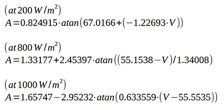
where A is the current, expressed in amperes; V is the voltage, expressed in volts; and atan is the arctangent function.
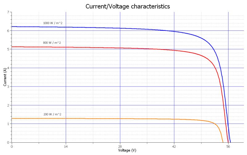
Figure 1: The graph of current on the characteristic voltage of the solar panel under observation
Obviously, the solar panel performs at a higher solar illumination, as can be seen from the power graph shown in Figure 2. The user should refer to this graph to assess the actual performance of their solar panel. Remember that power curves are always different, from solar panel to solar panel. By manually collecting the voltage and current values, using different resistive loads, one obtains more or less the same curves, even under the same lighting conditions. The graphs demonstrate, as mentioned above, the presence of a strong non-linearity.
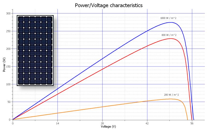
Figure 2: The power graph on the characteristic voltage of the solar panel under observation
If one wishes to find a simplified model (see the corresponding curve in Figure 3), one can adopt the segment model, for which it is sufficient to take the three fundamental points of the graph (e.g., with illumination of 1,000 W/m2), as listed below:
• Short-circuit current (characteristic point set at 0 V and 6.2 A)
• Current at maximum power (characteristic point set at 49.5 V and 5.54 A)
• No-load current or very light load (characteristic point set at 56.6 V and 0 A)
The relevant mathematical model is as follows:

where A is the current, expressed in amperes, and V is the voltage, expressed in volts.
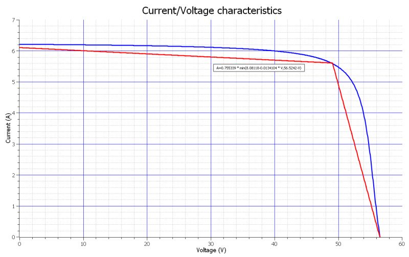
Figure 3: An approximation of the “current-voltage” response of the solar panel can be obtained using a segment model with three characteristic points (red graph).
The solar panel with LTspice
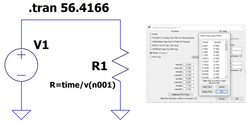
Once we have obtained the current-to-voltage characteristic of the solar panel, supplied with a light power of 1,000 W/m2, we can create an electrical diagram with LTspice that involves a voltage generator programmed with a sequence of data, corresponding precisely to the different voltage and current points of the device. To achieve this, the simulator’s functionality must be altered a little. In the circuit diagram, shown in Figure 4, a voltage generator in PWL mode is used with the following voltage and current value pairs:
PWL(0.2264,6.1084,2.1804,6.1045,4.5388,6.0964,7.7159,6.1023,10.6013,6.1086,13.4327,6.1087,17.5832,6.1194,21.0339,6.1298,24.5366,6.1365,29.6405,6.1432,33.3326,6.1386,36.791,6.1235,38.3397,6.1151,39.8958,6.0897,40.962,6.0762,42.0465,6.0442,42.9503,6.0192,43.9702,5.9791,44.7935,5.9482,45.8311,5.8931,47.6347,5.7612,49.3722,5.5612,51.0007,5.2754,51.8803,5.0397,52.5825,4.7801,53.3036,4.4215,53.5758,4.2184,53.8886,4.0168,54.245,3.6588,54.4233,3.4628,54.6171,3.2451,54.9128,2.8736,55.1341,2.483,55.2463,2.2524,55.3904,1.9954,55.5254,1.7288,55.7126,1.4244,55.9848,0.9462,56.1897,0.5251,56.2896,0.3061,56.4166,0.0502)
The value string is very long but can be entered very quickly in text form. As mentioned before, the value pair represents, respectively:
• The voltage value of the solar panel (as the first value)
• The solar panel current value (as the second value)
Although this is a simulation in the transient range (i.e., in the time domain), the following should be noted:
• The value of the abscissas does not represent time but is the voltage of the solar panel.
• The value of the ordinates does not represent voltage but is the current generated by the solar panel.
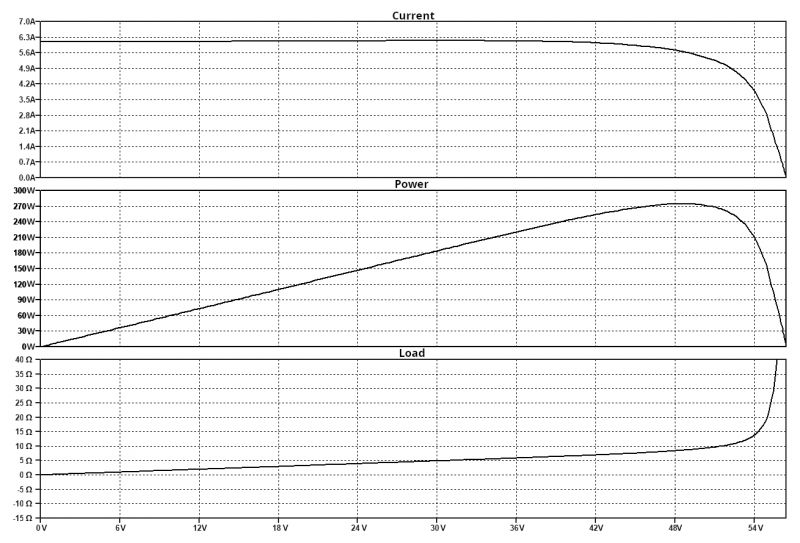
Figure 5
Therefore, the graphs in Figure 5 describe the following quantities:
• The first graph, at the top, represents the value of the circulating current.
• The second graph, in the middle, represents the value of the generated power.
• The third graph, at the bottom, represents the ohmic value of the equivalent resistive load.
It is interesting to note how the resistive value of the load is calculated using Ohm’s law, always remembering that the value of time is replaced by that of voltage and the value of voltage is replaced by that of current. It sounds a bit complicated, but this simple trick allows you to obtain optimal results from LTspice. The resistive value of the load, therefore, is described by the following strange formula:

Modeling a solar panel electrically can be a complex but useful process for predicting panel performance under specific operating conditions. There are several approaches to creating a model, such as the use of experimental data or the use of theoretical models. Regardless of the approach chosen, it is important to verify that the generated model is accurate and can be used to reliably predict solar panel performance. It can be used in a variety of applications, including solar system design, performance optimization and simulation of environmental conditions. As we have seen in this article, the electrical behavior of a solar panel can be simulated easily, provided that all voltage and current values are known, under various lighting conditions and applied loads.

Electrically modelling a solar panel
The electronic market makes thousands of solar panel models available to users. Each solar panel has its own electrical, physical and optical characteristics, so it is not possible to unify all the behaviors of such generators in one ideal device. One of the best methods to outline the electrical behavior of one’s solar panel is to collect measured experimental data to create a mathematical model. A solar panel does not have linear behavior, so the difficulty in generating the relevant equations may be greater. On the contrary, the solar panel is a highly non-linear element, so its behavior is comparable to a hybrid current generator (when the panel generates a low voltage due to strong loads) and a current generator (when the panel generates higher voltages due to light loads). It is therefore completely incorrect to equate the operation of a solar panel with a simple battery. For our analysis, we use a solar panel characterized by the following technical data:
• Maximum power: 250 W
• Open-circuit voltage: 37.8 V
• Short-circuit current: 8.7 A
• Maximum power voltage: 31.5 V
• Maximum power current: 7.94 A
• Module efficiency: 15.3%
• Operating temperature: between –40˚C and 85˚C
• Dimensions: 1,650 × 992 × 40 mm
• Weight: 17 kg
Figure 1 shows the graph of the current on the characteristic voltage. These values can also be deduced from practical measurements, with certain resistive loads applied to the solar panel itself. As shown in the figure, there are three separate graphs for three conditions under which the device is illuminated by the sun:
• 1,000 W/m2
• 800 W/m2
• 200 W/m2
The three curves can be summarized in as many mathematical models, which accurately express the course of current values as the voltage varies. The three simple models describing the current-voltage values of the solar panel, at the three lighting conditions, are as follows:

where A is the current, expressed in amperes; V is the voltage, expressed in volts; and atan is the arctangent function.

Figure 1: The graph of current on the characteristic voltage of the solar panel under observation
Obviously, the solar panel performs at a higher solar illumination, as can be seen from the power graph shown in Figure 2. The user should refer to this graph to assess the actual performance of their solar panel. Remember that power curves are always different, from solar panel to solar panel. By manually collecting the voltage and current values, using different resistive loads, one obtains more or less the same curves, even under the same lighting conditions. The graphs demonstrate, as mentioned above, the presence of a strong non-linearity.

Figure 2: The power graph on the characteristic voltage of the solar panel under observation
If one wishes to find a simplified model (see the corresponding curve in Figure 3), one can adopt the segment model, for which it is sufficient to take the three fundamental points of the graph (e.g., with illumination of 1,000 W/m2), as listed below:
• Short-circuit current (characteristic point set at 0 V and 6.2 A)
• Current at maximum power (characteristic point set at 49.5 V and 5.54 A)
• No-load current or very light load (characteristic point set at 56.6 V and 0 A)
The relevant mathematical model is as follows:

where A is the current, expressed in amperes, and V is the voltage, expressed in volts.

Figure 3: An approximation of the “current-voltage” response of the solar panel can be obtained using a segment model with three characteristic points (red graph).
The solar panel with LTspice
Once we have obtained the current-to-voltage characteristic of the solar panel, supplied with a light power of 1,000 W/m2, we can create an electrical diagram with LTspice that involves a voltage generator programmed with a sequence of data, corresponding precisely to the different voltage and current points of the device. To achieve this, the simulator’s functionality must be altered a little. In the circuit diagram, shown in Figure 4, a voltage generator in PWL mode is used with the following voltage and current value pairs:
PWL(0.2264,6.1084,2.1804,6.1045,4.5388,6.0964,7.7159,6.1023,10.6013,6.1086,13.4327,6.1087,17.5832,6.1194,21.0339,6.1298,24.5366,6.1365,29.6405,6.1432,33.3326,6.1386,36.791,6.1235,38.3397,6.1151,39.8958,6.0897,40.962,6.0762,42.0465,6.0442,42.9503,6.0192,43.9702,5.9791,44.7935,5.9482,45.8311,5.8931,47.6347,5.7612,49.3722,5.5612,51.0007,5.2754,51.8803,5.0397,52.5825,4.7801,53.3036,4.4215,53.5758,4.2184,53.8886,4.0168,54.245,3.6588,54.4233,3.4628,54.6171,3.2451,54.9128,2.8736,55.1341,2.483,55.2463,2.2524,55.3904,1.9954,55.5254,1.7288,55.7126,1.4244,55.9848,0.9462,56.1897,0.5251,56.2896,0.3061,56.4166,0.0502)
The value string is very long but can be entered very quickly in text form. As mentioned before, the value pair represents, respectively:
• The voltage value of the solar panel (as the first value)
• The solar panel current value (as the second value)
Although this is a simulation in the transient range (i.e., in the time domain), the following should be noted:
• The value of the abscissas does not represent time but is the voltage of the solar panel.
• The value of the ordinates does not represent voltage but is the current generated by the solar panel.

Figure 5
Therefore, the graphs in Figure 5 describe the following quantities:
• The first graph, at the top, represents the value of the circulating current.
• The second graph, in the middle, represents the value of the generated power.
• The third graph, at the bottom, represents the ohmic value of the equivalent resistive load.
It is interesting to note how the resistive value of the load is calculated using Ohm’s law, always remembering that the value of time is replaced by that of voltage and the value of voltage is replaced by that of current. It sounds a bit complicated, but this simple trick allows you to obtain optimal results from LTspice. The resistive value of the load, therefore, is described by the following strange formula:

Modeling a solar panel electrically can be a complex but useful process for predicting panel performance under specific operating conditions. There are several approaches to creating a model, such as the use of experimental data or the use of theoretical models. Regardless of the approach chosen, it is important to verify that the generated model is accurate and can be used to reliably predict solar panel performance. It can be used in a variety of applications, including solar system design, performance optimization and simulation of environmental conditions. As we have seen in this article, the electrical behavior of a solar panel can be simulated easily, provided that all voltage and current values are known, under various lighting conditions and applied loads.


