Physical values cannot be determined with absolute certainty. Tools and measuring systems always have a certain tolerance and are not fully immune to disturbances that introduce a certain degree of uncertainty into the measurement. When it comes to uncertainty of measurement, the following terminology is often used:
*
Offense or absolute error measurement - the difference between the real value and the measured value (in the following parts of the text, for the sake of simplicity, we will use the term
accuracy - note red);
*
Variance - a measure of the size of a random distribution of measured values around the expected value (we will use the term
precision - note ed.);
*
Resolution - value of the smallest, distinguishable by the measuring system change of the real value of the measured parameter.
In practice, these terms are often used inaccurately or even interchangeably - it is significant that the resolution and accuracy (in terms of variance or standard deviation) of the measurement are used interchangeably. In the following article, we will briefly discuss these concepts.
Measurement uncertainty Measurement uncertainties can be divided into systematic and random errors. Systematic errors are caused by deviating from ideal measuring instruments, i.e. errors in measurement, gain, offset, etc. of measuring tools. Random errors, in turn, are caused by noise and induced voltages or currents in the system.
Accuracy and precision of definitions Accuracy and precision are often used interchangeably; are considered synonyms. However, the two terms have a completely different meaning. Accuracy indicates how close a measurement value is to the true value of a given value, ie what is the deviation between the measured and actual values. Precision refers to the random distribution of the measured values.
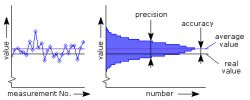
Fig. 1. Definitions of uncertainty. On the left
side of a series of measurements. On the right
values in the histogram.
After taking a series of measurements of a stable voltage or other parameter, the measured values will show some variation. This is due to, inter alia, thermal noise in the circuits of the measuring equipment and the rest of the measuring system. Left graph on
Figure 1 illustrates this variability.
Histogram The measured values can be plotted on the histogram as shown in
Figure 1 . The histogram shows how often a given value occurs in a measurement. The highest point of the histogram, i.e. the most frequently obtained value in the measurement, usually indicates the average value. This is indicated by the blue line in both charts. The black line represents the actual value of the parameter. The difference between the average measured value and the actual value is the accuracy. The width of the histogram shows the distribution of the individual measurements. This distribution of measurements speaks of the precision of the measurement.
Use correct definitions Accuracy and precision therefore have two different meanings. It is therefore quite possible that the measurement is very precise, but it is not at all accurate; or vice versa - a very accurate measurement does not have to be precise at all. In general, a measurement is considered correct if it is accurate and precise.
Accuracy Accuracy is one of the characteristics that indicates the correctness of a measurement. Since precision also affects accuracy with a single measurement, the average of the series of measurements will be taken.
The uncertainty of a measuring instrument is usually given by two values: reading uncertainty and uncertainty for the full scale (full measuring range). Together, these two specifications define the overall uncertainty of a given measurement. Measurement uncertainty values are given as a percentage or ppm (parts per million) of the current national standard. 1% corresponds to 10,000 ppm.
The given uncertainty is determined both for specific ranges of operating temperatures and for a specified period of time after calibration of the device. Also note that different uncertainty values may apply for different measuring ranges.
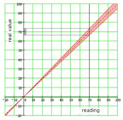
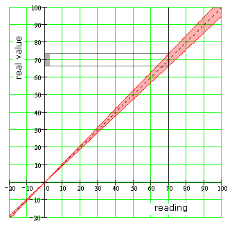
Fig.2. Reading uncertainty 5% at
reading value 70 V.
Uncertainty related to reading An indication of the percentage deviation without further specification also applies to the reading. Voltage divider tolerances, gain accuracy, absolute reading deviation or digitization (quantization) of the measured value all contribute to this inaccuracy.
A voltmeter that reads 70.00 volts and has a specification of "? 5% of reading" will have an uncertainty of 3.5 volts (5% of 70 volts) above and below the measurement. The actual voltage will therefore be between 66.5 and 73.5 volts, which can also be written as (70.00 ? 3.50) V.
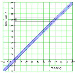
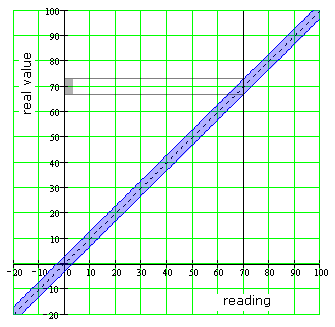
Fig. 3. 3% full scale uncertainty
in the range of 100 V.
Uncertainty expressed relative to the full scale This type of inaccuracy is caused by offset errors and linearity errors in the amplifiers, as well as - in systems where the measured value is digitized - the non-linearity of the analog-to-digital conversion and the uncertainty of the ADC itself.. This specification applies to the full measuring range of the system.
For example, a voltmeter may have a "3% full scale" specification. If 100V range (ie full scale) is selected during measurement, the uncertainty is 3% from 100V = 3V regardless of the voltage measured. If the reading within this range is 70 volts then the actual voltage is 67 to 73 volts - (70 ? 3) volts.
Picture nr 3 explains that the type of tolerance is independent of the value read. If 0 volts were measured in this way, the voltage might actually be -3 to +3 volts - (0 ? 3) volts.
Uncertainty over the full range of work expressed in 'numbers' Often times, a digital multimeter measures the complete uncertainty in terms of the number of significant digits instead of a percentage. Digital multimeter with 3 1/2 digit display (range -1999 to 1999), the specification can read the uncertainty value as "+ 2 digits". This means that the display uncertainty is 2 units. For example: if the range is 20 volts (? 19.99V), the full scale uncertainty is ? 0.02V. The display shows 10.00V, which means the actual value is (10.00 ? 0.02 ) V.
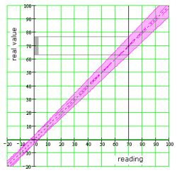
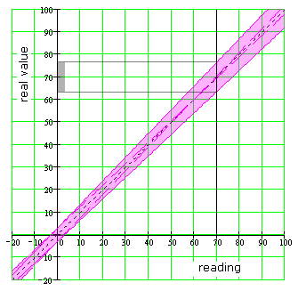
Pic.4. Total uncertainty 5%
reading and 3% of full scale for
100V range and 70V reading.
Calculation of measurement uncertainty The specification of the reading tolerance and full scale together define the overall measurement uncertainty for a given instrument. The following example uses the same values as the examples above, that is:
* Accuracy: ? 5% for reading and 3% of full scale;
* Measuring range: 100V;
* Reading range: 70V
The total measurement uncertainty is now calculated as follows:
$$\frac {\%odczytany} {100%} \times odczyt = \frac {5\%} {100%} \times 70 V = 3,5 V$$ $$\frac {\%Pełnej\ skali} {100%} \times zakres = \frac {3\%} {100%} \times 100 V = 3 V \qquad (1)$$ $$3,5 V + 3 V = 6,5 V$$ In this situation, the total measurement uncertainty is therefore 6.5V up and down. The actual value is therefore in the range from 62.5 V to 77.5 V.
Picture nr 4 it illustrates graphically.
Percentage uncertainty is the relationship between the reading and the uncertainty. In this situation it is described
equation 2 :
$$\frac {niepewność} {odczyt} \times 100\% = \frac {6,5 V} {70 V} * 100% = 9,29% \qquad (2)$$ Number of digits for the device Digital multimeters may include the specification "? 2.0% rdg, + 4 digits." This means that "4 digits" must be added to the reading uncertainty of 2%. Let's use a 3 1/2 digit multimeter again as an example. It reads 5.00V while the range is 20V. 2% of the reading would mean an uncertainty of 0.1 V. Add in the digit inaccuracy (= 0.04 V). The total uncertainty is therefore 0.14 V. The actual value should therefore be (5.00 ? 0.14) V.
Resultant total uncertainty of measurement Often only the uncertainty of the measuring instrument itself is taken into account. However, care should also be taken to take into account the additional measurement uncertainty of the measuring accessories used, if they are used. Here are some common examples:
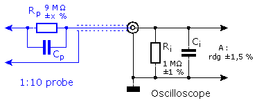
Increased uncertainty when using a 1:10 oscilloscope probe When a 1:10 probe is used, not only the measurement uncertainty of the instrument itself should be considered. The input impedance of the instrument used and the probe resistance, which together form the voltage divider, also have an influence on the uncertainty.
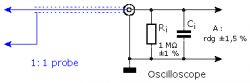
Pic.5. 1: 1 probe used for measurement.
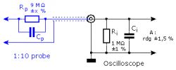
Pic. 6. 1:10 probe connected to
the oscilloscope introduces an additional one
uncertainty for measurement.
Picture nr 5 schematically shows an oscilloscope with a 1: 1 probe. If we find this probe ideal (no series resistance), the voltage applied to the probe is passed directly to the oscilloscope input. The measurement uncertainty is now determined only by the tolerances in the attenuator, amplifier and further processing in the oscilloscope, and is specified by its manufacturer. The uncertainty is also influenced by the resistive network which forms the internal resistance Ri. This is taken into account within the tolerances specified by the manufacturer.
Picture nr 6 shows the same measuring range, but now the probe used is 1:10. This probe has an internal series resistance of Rp and forms a voltage divider with the oscilloscope input resistance Ri. The tolerance of the resistors in the voltage divider will cause the test probe to add its own non-zero uncertainty.
The tolerance of the oscilloscope input resistance can be found in the oscilloscope specifications. Series resistance Rp tolerance of a probe is not always given in its documentation. However, the uncertainty of the measurement system as determined by the connection of the oscilloscope probe to a particular type of oscilloscope will be known. If the probe is used with a type of oscilloscope other than that recommended, the measurement uncertainty is not specified. This situation should be avoided in the case of precise measurements.
Root of the sum of squares To obtain the resulting measurement uncertainty, all component tolerances should be summed as the root of the sum of the squares. In the example below, the oscilloscope has a tolerance of 1.5% and the 1:10 probe used has a measurement uncertainty of 2.5%. These two specifications must be summed - the square root of the sum of the squares is used for this. This is shown on
equation 3 below.
$$ \%total = \sqrt {\%odczyt ^2 + \%systemowy ^2} = \sqrt {1,5^2 + 2,5^2} \approx 2,915\% \qquad (3)$$ 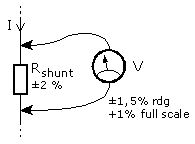
Pic.7. Increasing uncertainty
when using the actual
a resistor to measure the current.
Current measurements with the help of a measuring resistor Often, a measuring resistor is used to measure the value of the flowing current. The current flowing through this element causes a certain voltage drop on it, which can be easier measured using, for example, a multimeter or an oscilloscope. The tolerance of this resistor translates into the measurement uncertainty of this system. Knowing it and the measurement uncertainty of the device used in the further part of the measurement, it is possible to estimate the total measurement uncertainty with the help of the square root. It was presented on
equation 4 :
$$ \%total = sqrt {\%odczyt^2 + \%opornik^2} = \sqrt {1,5^2 + 2^2} \approx 2,5\% \qquad (4)$$ In this example, the overall reading uncertainty is 2.5%.
The shunt resistance is additionally dependent on the temperature. The resistance value is specified for a certain standard temperature. Temperature dependence - the temperature coefficient of resistance - is often expressed in ppm / ° C and tells how the electrical resistance of a resistor changes as its temperature changes. As an example, a resistance value at ambient temperature (Tamb) of 30 ° C was calculated. The used measuring resistor is characterized by the nominal resistance R = 100 ? at the temperature of 22 ° C (these are the parameters Rnom and Tnom). The element temperature coefficient of resistance is 20 ppm / ° C. The actual resistance calculations are shown in
equation 5 .
$$ ( 1 + (T_{amb} - T_{nom}) \times \frac {ppm} {1000000}) \times R_{nom} = ( 1 + (30 - 22) \times \frac {20} {1000000}) \times 100 = 100,016 \Omega \qquad (5)$$ The current flowing through the shunt dissipates energy, which in turn leads to an increase in temperature and thus a change in the resistance value. The change in resistance value due to current flow depends on several factors. For very accurate measurements, the shunt should be calibrated at the specific resistance, current flow and environmental conditions in which it will be used.
Precision Deadline
precision is used to express a random error of measurement. The random nature of the measured value deviations is mainly of a thermal origin in the case of electronic systems. Due to the arbitrary nature of this noise, an absolute error cannot be given. Precision only gives the probability that the measurement value is within the stated limits.
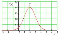
Fig 8. Probability distribution
for ? = 2 and en ? = 1.
Gaussian distribution Thermal noise has a Gaussian distribution called the normal distribution. It is described by the following equation:
$$f(x) = \frac {1} {\sigma \sqrt {2 \times \pi}} \times exp (\frac {-(x-\mu)^2}{2 \times \sigma^2}) \qquad (6)$$ where ? is the mean value and ? indicates the degree of scattering and corresponds to the RMS value of the noise signal. This function provides a probability distribution curve as shown in
figure 8 , where the mean value of ? = 2 and the effective noise amplitude ? = 1.
Probability table Some values for the probability of finding a value are listed in the table below, expressed at a certain level. As you can see, the probability that the measured value is within ? 3? is 99.7%, therefore most calculations use 3? as the width of the "whole" distribution.
| Range | Probability |
| 0.5 ? | 38.3% |
| 0.674 ? | 50.0% |
| 1 ? ? | 68.3% |
| 2 ? ? | 95.4% |
| 3 ? ? | 99.7% |
Improving the precision Measurement precision can be improved by oversampling or filtering. The individual measurements are averaged so that the amount of noise is significantly reduced. The range of the measured values is thereby also reduced. When oversampling or filtering, it should be considered that this can reduce the throughput of the measurement system.
Resolution The resolution of the measuring system is the smallest difference between the values distinguishable by the system. Determining the resolution of an instrument is not related to its measurement accuracy.
Digital measuring systems The digital system converts an analog signal into a digital equivalent with the help of an analog-to-digital converter (ADC). The difference between two "adjacent" values in a quantized signal is called resolution, and it is always equal to one bit in the digital signal. For a digital multimeter, it is one digit.
It is also possible to express the resolution in units other than bits. For example, a digital oscilloscope with an 8-bit ADC - if its vertical sensitivity is set to 100 mV / div and the number of divisions is 8, the total range will be 800 mV. 8 bits represent 2 ^ 8 = 256 different values. The resolution in volts is then 800 mV / 256 = 3.125 mV.
Analog measuring systems For analog measuring instruments where the measured value is displayed mechanically, such as a moving coil gauge, it is difficult to give an exact value for the measurement resolution. First, the resolution is limited by the mechanical hysteresis of the system due to the friction of the needle bearings. On the other hand, the resolution is also determined by the observer, making it very subjective to judge.
Source:
https://meettechniek.info/measurement/accuracy.html 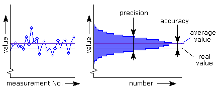


Comments
Until I don't want to drag everything out. Total error instead of "total" (total), not the reading but the indicated value, and please do not struggle once with a resistor and once with a resistor.... [Read more]
Translation like translation. Specification "3% full scale" translated as "3% full scale" specification has always been called the meter class. After translation, he can correct the text based on Polish... [Read more]